Model and Response Function

Introduction

In marketing, models are essential tools for understanding, predicting and optimizing the impact of marketing actions on business results. A fundamental element of these models is the response function, which describes the relationship between marketing efforts and the results obtained.

What is a response function?

A response function in marketing is a mathematical representation of the relationship between one or more input variables (usually marketing efforts) and an output variable (usually a performance measure such as sales, market share, or return on investment).

Types of response functions

1. Linear function
   • The simplest, it assumes a directly proportional relationship between effort and result.
   • Equation: Y = a + bX where Y is the result, X is the marketing effort, a is the y-intercept, and b is the slope.
2. Logarithmic function
   • Reflects diminishing returns as effort increases.
   • Equation: Y = a + b * log(X)
3. Exponential function
   • Models rapid initial growth followed by a plateau.
   • Equation: Y = a * (1 – e^(-bX))
4. S function (sigmoid)
   • Combines slow initial growth, acceleration, then slowdown.
   • Equation: Y = a / (1 + e^(-b(X-c)))

Practical example: Ad response function

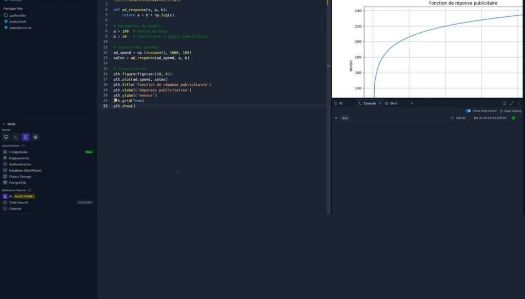
Let’s imagine we want to model the impact of advertising expenditure on the sales of a product. We’ll use a logarithmic function to reflect the diminishing returns often observed in advertising.

Here is an example of Python code to visualize this response function:

import numpy as np
import matplotlib.pyplot as plt

def ad_response(x, a, b):
    return a + b * np.log(x)

# Paramètres du modèle
a = 100  # Ventes de base
b = 20   # Coefficient d'impact publicitaire

# Générer des données
ad_spend = np.linspace(1, 1000, 100)
sales = ad_response(ad_spend, a, b)

# Visualisation
plt.figure(figsize=(10, 6))
plt.plot(ad_spend, sales)
plt.title('Fonction de réponse publicitaire')
plt.xlabel('Dépenses publicitaires')
plt.ylabel('Ventes')
plt.grid(True)
plt.show()

This code creates a graph showing how sales increase as a function of advertising expenditure, with decreasing returns.

Application in Excel

For those who prefer to work with Excel, here’s how you might structure a spreadsheet to model this response function:

1. Column A: Advertising expenditure (from 0 to 1000, in increments of 50)
2. Column B: Response function formula
   • Cell B2: =100 + 20*LN(A2)
3. Draw a scatter plot with expenses on the X axis and sales on the Y axis.

Interpretation and use

1. Elasticity: The slope of the curve at a given point represents the elasticity of the response. It indicates the marginal change in sales for a change in advertising expenditure.
2. Optimization: By analyzing the curve, marketers can identify the point at which yields start to fall significantly, helping to optimize the advertising budget.
3. Forecasting: Once calibrated with real data, the model can be used to forecast the impact of different levels of advertising spend.

Limits and considerations

• Simplified response functions don’t capture the full complexity of the real market.
• Other factors (competition, seasonality, etc.) can influence the relationship.
• It is crucial to regularly recalibrate the model with new data.

Conclusion

Response functions are a fundamental tool in marketing modeling. They quantify and visualize the impact of marketing efforts, facilitating decision-making and resource optimization.